Fiji Plugin
The B-recs package provides a plugin for Image J / Fiji. Once installed, you can find the functions under the menu Plugins > B-recs.
PSF generator
B-recs uses PSF images in a particular format. In order to ease the use of B-recs, you can generate a simple gaussian PSF via this function. Note however that it is always better to produce a PSF that is specifically designed to fit the real PSF of your optical system. You need to enter a few parameters to produce the PSF:
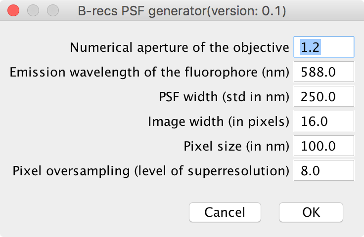
Numerical aperture of the objective Enter here the numerical aperture of your objective. Typical values are between 0.8 and 1.3.
Emission wavelength of the fluorophore (nm) Emission wavelength of your fluorophore (509 nm for GFP).
PSF width (FWHM in nm) If you don’t know the value of the PSF width, you can enter instead the numerical aperture of your objective and the emission wavelength of your fluorophore of interest. The width of the PSF will then be automatically updated with the formula:
\[FWHM = 0.4\, \lambda\, /\, NA\]Image width (in pixels) Size of the PSF. This has to be a multiple of 8. It should be as small as possible (to increase the processing speed) while retaining all the extent of the PSF. In practive, it is either 8 or 16.
Pixel size (in nm) Enter here the size of your camera pixels relative to your sample size: if the physical size of your camera pixel is 10 µm and the magnification of your objective is 100 px, you should enter here 10 µm / 100 = 100 nm.
Pixel oversampling (level of superresolution) Ratio of the number of pixel of the reconstructed image over the number of pixel of the measured image. If your pixel size is 100 nm and you expect a effective superresolution of 20 nm, you should enter 5 here.
Once generated, you will see a stack of images appear in Image J. This stack can be readily used for the 2d reconstruction.
2D reconstruction
This is the core of the plugin. The parameters are slightly trickier to tune. If a set of parameter do not lead to a reasonable output, a few guidelines are given at the end of this paragraph.
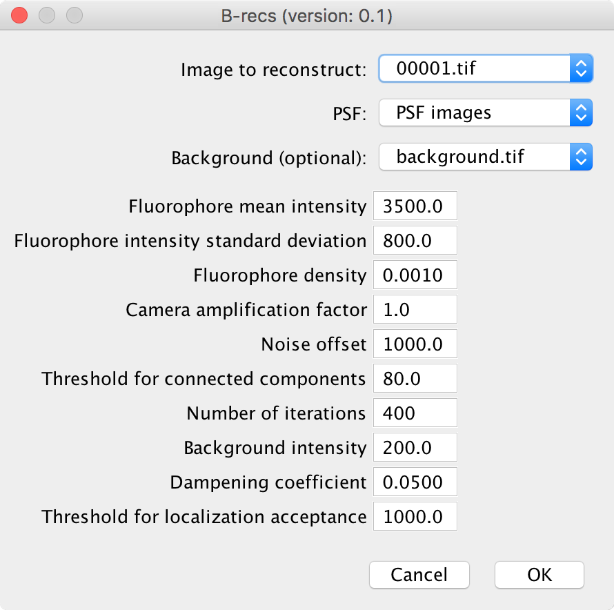
Dataset This is where you provide an image to reconstruct. The image has to be in grayscale, in 16 bits format.
PSF You can directly put here a PSF in the format generated by the PSF generator function of the plugin.
Background It is possible to provide an image which gives the background level of each measured pixel. Typically this is an average over all the measured image or alternatively, an image measured after the sample is all bleached out. A more straightforward way to otain the background level but which is less accurate in the case of a very dense sample is to take the median over the whole stack of images to reconstruct. This parameters can also help with taking into account the different levels measured when not sample is present (this is typically the “hot” pixels observed with CMOS cameras). Hence, for CMOS cameras, the Background parameters can be an image acquired when the shutter is present.
Fluorophore mean intensity Mean number of photons emitted by a fluorophore. In the simplest mode where the distribution of the number of emitted photons is gaussion, this is the mean of this distribution. A typical number is 2000 photons.
Fluorophore intensity standard devitation This the standard deviation of the gaussian distribution of the number of emitted photons. Again, a typical number is 300. The prior of the intensity of each reconstructed pixel is given by:
\[\psi(I) = (1 - \rho) \delta(I) + \frac{\rho}{\sqrt{2 \pi \sigma ^2}} \exp\left(-\frac{(I - I_m)^2}{2 \sigma^2}\right)\]\(\rho\): density of fluorophores
- \(I_m\): mean number of photons emitted by a fluorophore (fluorohore
mean intensity parameter).
- \(\sigma\): standard deviation of this number of photons (fluorophore
intensity standard deviation parameter).
Fluorophore density This is the \(\rho\) parameter of the previous equation
Camera amplification factor The input image is a grayscale image. The intensity of each pixel can be directly expressed in number of photons. In that case, the amplification factor would be 1. Otherwise, it is possible, as is often the case for CCD cameras, to have an amplification factor which gives the mean ration of the image intensity over the number of photons. A typical value for CCD cameras is 10.
Noise offset The noise model for the detected photons is linear: \(\sigma = a + b * I\) It means that there is a constant level of noise added to the expected photon shot noise of the measurement. The noise offset parameter is the factor a. It typically gives the level of the electronic noise of the detector. The factor b comes from the Poisson distribution and is equal to 1.
Threshold for connected components In order to speed up the algorithm, the image regions where the intensity is close to the background, and hence where fluorophore are absent are not taken into account. This threshold is the intensity level above the background that indicates the presence of a fluorophore. It is typically a few standard deviation of intensity distribution around the background.
Number of iterations It happens very often that because of non-modelled noise in the image, the algorithm has trouble to fully converge. This parameter indicates the number of iterations after which B-recs stops whatever the level of convergence is.
Background intensity If no image is provided for the background intensity, it is still possible to assume a uniform background level. This is this level in number of photons.
Dampening coefficient In order to help the algorithm to converge, the update of a posteriori intensities is dampened. This coefficient should be below one. Generally a coefficient equal to one leads to instabilities in the algorithm (it is easy to detect it a posteriori in the geconstructed images). A coeffecient 0.01 is on the safe side (but slow). I usually use 0.05 for 2D datasets.
Threshold for localization acceptance After the algorithm run, you obtain an image gives the posterior superresolved intensities. From this image, it is possible to obtain a list of localization by thresholding. This thresholding value is the value of the intensity in the reconstructed image beyond which localizations are considered.
Guideline for the use of parameters
A really important parameter is the level of noise of the pixel. A common mistake when using B-recs is the use a too low noise level. This will result in B-recs assuming that details in the pictures should be accounted for by florophore photons instead of background noise and make these levels inconsistent the the PSF used. The algorithm in that scenario will always have trouble to find something significant. It is always better to try with a high level of noise first and the increase it progressively until obtaining reasonable results. This problem should arise if you perfectly control your optical and measurement system but this rarely completely occurs.
In the case you miss some of the spots, it could mean that the background level you set was to high. Alternatively, it could mean that the distribution of the number of photons emitted by a fluorophore is not set correctly (ie a too high mean number of photons coupled with a too narrow standard deviation will tend to miss many spots). The opposite of the previous tendencies will lead to the apparison of many spurious spots.
Test dataset
A good dataset to test B-recs is provided by the ISBI challenge 2013
[ISBI2013].
The necessary files with the preprocessed datasets are available in the
test folder of the B-recs package.
ISBI dataset 1
The dataset 1 (in low density) has a background that is correlated in time and
space but not constant over the whole acquisition time. A simple idea to remove
the background in that case is to use a median filter in x, y and t with a
radius of 4 pixel in every plane direction and 2 pixels in t.
The resulting stack is called background.tif.
Removing this background from the measured images, and collecting the total
intensity around a few spots allows to determine the distribution of the number
of emitted photons (see the table below). Notice that it is also a good idea to
use a first guess and to refine this parameters a posteriori on the
localization intensities after a few runs.
Then by plotting the histogram of the intensities (again after the background
is removed), it is easy to determine a reasonable threshold for the connected
components determination: it is the upper value of the background distribution.
The dampening coefficient is the one I almost always use for 2D
reconstructions.
Here is set of parameters that give reasonable results:
| Fluorophore mean intensity | 3500 |
| Fluorophore intensity standard deviation | 800 |
| Fluorophore density | 0.001 |
| Camera amplification factor | 1.0 |
| Noise offset | 1000 |
| Threshold for connected components | 80 |
| Number of iterations | 400 |
| Dampening coefficient | 0.05 |
| Threshold for localization acceptance | 1000 |
And for the PSF:
| PSF width (FWHM in nm) | 260.0 |
| Image width (in pixels) | 8 |
| Pixel size (in nm) | 100.0 |
| Pixel oversampling (level of superresolution) | 8 |
The current version of the plugin do not allow for a progress bar. It should take no longer than a few seconds to reconstruct an image.
| [ISBI2013] | Sage, D., Kirshner, H., Pengo, T., Stuurman, N., Min, J., Manley, S., & Unser, M. (2015). Quantitative evaluation of software packages for single-molecule localization microscopy. Nature methods, 12(8), 717-724. |